Seasonality analysis

Freight modeling is currently a very hot topic in the US, and California currently has its CSFFM being developed at UCI by a team to which I belong.

First of all, there are two main streams of freight modeling. The first one has a more urban accent to it, and usually models truck movements, like the one used by SCAG. The second type is a commodity-based model, like our very own CSFFM.

For commodity-based models there are two main possible data sources: FAF and Transearch. While Transearch can have much more detail on both temporal and spatial scales, FAF is very aggregate spatially and presents only yearly commodity flows. As Transearch is quite expensive and it was deemed not worth its cost for the project’s purpose (the reasons are unimportant here), CSFFM is being based on FAF (which is free).

Even though CSFFM is based on yearly flows, we would need to, ideally, compute flows for the peak hour to be able to integrate it to the passenger model, CSTDM, currently being updated.

This type of conversion is usually made by the use of some sort of reference peak factor, which varies state by state and is usually applicable to truck flows, and are not commodity specific.

It is quite obvious that a flat factor would not reproduce the highly seasonal behavior of agricultural products, hence it was necessary to compute seasonality factors for distributing the yearly movements of agricultural products into smaller periods of time.

As I could not find ANY literature on how to proceed on this task, I had to come up with my own procedure. Basically, I used information on crops from USDA in three different formats: Raster images from remote sensing technology, agricultural census, and surveys.

The most important data source was CropScape, which is a remarkable database of crops for every square inch of the contiguous 48 states for several years. It has all the caveats that data coming from remote sensing technology has, but concerns with a bias on the data collection are very reduced (please read their FAQ for additional information).

The other data source used (combines surveys and census) was QuickStats, which is a more sparse data source, but still very useful. The result of the analysis was a distribution with the proportion of production for each day in each County in California (if can be reduced to areas much smaller than that due to the high resolution of the maps from CropScape).

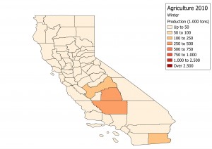
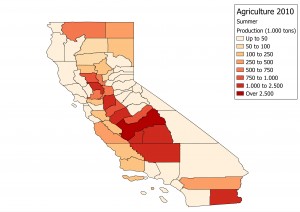
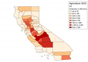
As the tables are hard to analyze, I’ll show a few maps for the 4 seasons.. It is quite clear the distinction, and proves the hypothesis that using a fixed factor would be inadequate to this case.

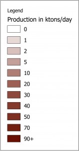
Production_Winter Production_Summer Production_Fall

Another interesting result I was able to produce was a video made with a sequence of 365 maps, showing how each County’s production evolves during the year.